State system behind the scenes

Salt state processing

Looking into the processing of Salt state files we see that:

• The Salt state system is composed of stages.

• Execution of a state runs through a series of stages.

• The stages provide levels of abstraction.

• The State system inside Salt is fundamentally data-driven.

• Each stage has a corresponding process for refining the initial data structure.

The stages and data layers of the Salt state system are shown in the following image:

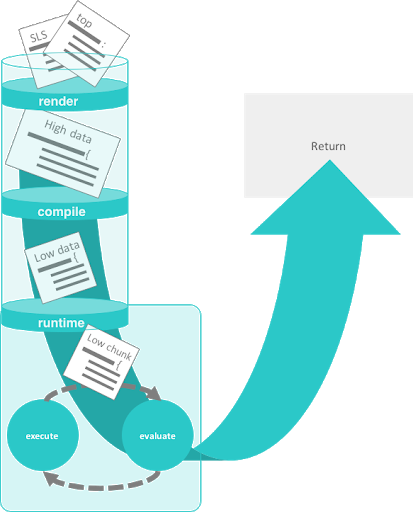
Stages of Salt state execution

In the Salt state system, there are three distinct stages of execution:

• the render

• the compile

• the runtime

Each stage manipulates the data in a way that allows for the states to be expressed dynamically . The entire process converts of all of the data down into a single pass static data structure.

State rendering

The render time is when the renderer engines are used. The top file and SLS files are converted into raw, unrefined high data. The process of state execution begins with the execution of a high state.

High state

Calling SLS directly logically assigns what states should be executed from the context of the calling minion. The Highstate layer is used to allow for full contextual assignment of what is to be executed tied to one or more minions from the master.

This means that the environment of a minion, and all associated execution data pertinent to said minion, can be assigned from the master without needing to execute or configure anything on the target minion. This also means that the minion can independently retrieve information about its complete configuration from the master.

The top file

In Salt, the file which contains a mapping between groups of machines on a network and the configuration roles that should be applied to them is called a top file.

Top files are downloaded from the master.

• The top files from each environment are downloaded and passed through the render interface.

• The top files are rendered. Top files can be processed by multiple renderers such as Jinja and YAML renderers.

The master_tops function is called.

• This function requests the master tops plugin interface from the master.

• The master evaluates all configured master tops plugin interfaces.

This pluggable interface allows for storing top file information in a database or via a provisioning tool. The top file routine generates the first data structure needed to kick off the state process.

Match evaluation

The matches dictionary contains all of the needed data to start gathering SLS references. A raw matches dictionary will be a variation of this format:

{'base': ['dns', 'dns.bind-utils','core', 'httpd', 'edit']}

Note

When calling state.sls the matches dictionary is generated from the SLS references s and the environment name sent as arguments to the function.

SLS rendering and templating

1. Each SLS file is rendered and the “raw” high data of that individual file is returned. The default renderers are the Jinja + YAML (yaml_jinja) renderers.

2. The templates in the file rendering sequence are all executed at this point. This means that all references to Salt functions are resolved now, before any execution of states begin.

3. As the SLS references are downloaded and rendered, their respective data is combined into a single Python dictionary which will be further processed.

The following image shows where rendering happens in the state execution process:

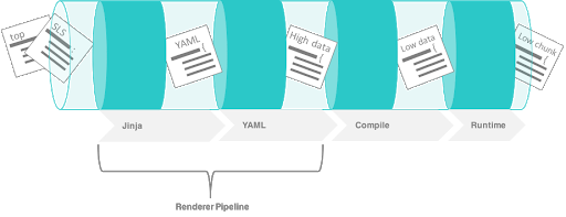
Rendering pipeline in the stages of state execution. This example shows the data conversion of a state when rendered and templated.

The following state fragment is written in YAML with a Jinja template expression to get the os_family grain:

named_conf:
  file.managed:
    - source: salt://dns/files/{{grains['os_family']}}-named.conf
    - name: /etc/named.conf

If the following state is rendered on a RedHat minion then it will be converted to:

named_conf:
  file.managed:
    - source: salt://dns/files/RedHat-named.conf
    - name: /etc/named.conf

High data

High data is the data structure represented in YAML via SLS files. The High data structure is created by merging the data components rendered inside SLS files (or other render systems).

The High data can be easily viewed by executing the state.show_highstate or state.show_sls functions. Since this is a somewhat complex data structure, it may be easier to read using the json, yaml, or pprint outputters:

salt '*' state.show_highstate --out yaml

salt '*' state.show_sls edit.vim --out pprint

Evaluation of include statements

If a single SLS file contains an include declaration, then the included SLS references need to be rendered. For each rendered SLS file with includes, the list of includes is read and the SLS references defined are resolved.

This is the point where include statement globs are reconciled.

• This means that the referenced includes are downloaded and rendered as they are found.

• The render sequence maintains which SLS references have already been downloaded ensuring that the same SLS file is not rendered twice.

Injected data

At a number of points in the compiler, data is injected into the structures for ordering and tracking needs. These injections enable many features of the runtime and are used to help pass the correct debug data up the chain.

Injected state auto order

While the order flag is inserted here, it has not been evaluated yet, which happens when the high data is compiled to low data. The YAML renderer has been modified to use ordered dictionaries instead of standard unordered dictionaries.

• This means that as the files are rendered that the order is preserved and order flags can be inserted into the state declarations.

• The order of the automatic state ordering is started at the tail-end of the include statement.

• Therefore, the first SLS file to get pushed into the high data dictionary is the first to get ordered.

• More simply put, the order is first declared at the end of the include chain.

• So, if SLS file ‘a’ includes file ‘b’, which includes file ‘c’, then the states in ‘c’ will be the first to be evaluated, then ‘b’ then ‘a’.

If the order is declared then it is honored, otherwise, a value is injected:

named_conf:
  file.managed:
    - name: /etc/named.conf
    - order: 10002  # <- order injected

start_bind:
  service.running:
    - name: named
    - order: last  # <- explicitly declared, not evaluated till later

Injected __sls__ and __env__ values

The SLS reference to the loaded file and the environment that file came from are both loaded into the state declarations at this point. These keys are called:

• __sls__ for the SLS reference

• __env__ for the environment

These values are read in by a number of states to ensure that the same environments are used to download source files as the SLS file was retrieved from:

named_conf:
  __env__: base # <- injected
  __sls__: dns  # <- injected
  file.managed:
    - source: salt://dns/files/RedHat-named.conf
    - name: /etc/named.conf
    - order: 10002

Start_bind:
  __env__: base  # <- injected
  __sls__: dns   # <- injected
  service.running:
    - name: named
    - order: last

Stashing extend and exclude statements

All extend and exclude statements are, at the time of each file being rendered, stashed into high-level data structures:

• __extend__ for extended states

• __exclude__ for excluded states

These structures maintain this data to be reconciled once all SLS references have been rendered. This means that all “top level” declarations are pulled out and combined during the initial rendering of the file.

Unrefined data

Once all of the SLS references have been rendered, the resulting data structure is the unrefined high data. The unrefined high data needs to be refined, reconciled, and then compiled.

The data structure shortcuts are cleaned up and the standard high data is made ready. This includes taking care of “short decs”, or dot delimited references. This cleanup changes all references that look like these:

named_conf:
  __env__: base
  __sls__: dns
  file.managed:
    - source: salt://dns/files/RedHat-named.conf
    - name: /etc/named.conf
    - order: 10002

start_bind:
  __env__: base
  __sls__: dns
  service.running:
    - name: named
    - order: last

Into structures that have removed the dot-delimited short decs:

named_conf:
  __env__: base
  __sls__: dns
  file:
    - managed  # <- function moved here
    - source: salt://dns/files/RedHat-named.conf
    - name: /etc/named.conf
    - order: 10002

start_bind:
  __env__: base
  __sls__: dns
  service:
    - running  # <- function moved here
    - name: named
    - order: last

All exclude top level declarations are now evaluated.

State compile

• The data is read for exclude matches and the respective excludes are pulled out.

• The main caveat to executing the excludes at this point is that this evaluation is after the includes.

• The result is that when states included from one file and excluded from another, the exclude will override the include.

State compile

Now that the state has been rendered it is ready to compile. The Salt state compiler consists of the reconciliation of complex raw high data structures:

• conversion of _in declarations to counterparts

• evaluate use declarations

• handle prereq declarations

• reconcile extend statements

• handle name references

• compile to low data (low chunks)

The following image shows state compiler routines

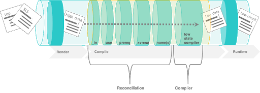
Reconciliation

State reconciliation includes:

• Reconcile complex raw high data

• Convert requisite_in declarations to requisites

• Use reconciliation

• Prereq fork reconciliation

• Handling extend

Reconcile requisite_in statements

The raw high data is scanned for requisite_in statements. The requisite_in statements that are found become transformed into data in the __extend__ structure to be evaluated next.

• An example of a requisite_in is require_in or watch_in

• The require_in and watch_in requisites are the simplest.

• These convert into extended data that applies the respective require and watch statements.

• The use and use_in requisites search through the high data for the redirected data and set the extended dictionary to apply the variables that will be used.

Reconcile prereq statements

The prereq system creates a fork.

• The problem is that prereq needs to apply a requisite to the thing which it requires while also soft requiring it.

• The prereq system therefore creates what is a recursive loop of requisites with an exit condition.

• The prereq sets all states which are pre-required with the pre-required requisite, while maintaining the prereq requisite.

• Other requisite_in``s dispose of the ``requisite_in statement because they are no longer needed, but the prereq statement is used in the runtime.

Reconcile extend statements

The extend statements are now reconciled.

State Compile

• The extend and requisite_in statements have now populated the __extend__ dictionary in the raw high data.

• Each key in the __extend__ dictionary is now evaluated and lined up with the respective dictionary key in the raw high data.

• The extend statements are then used to modify the raw high data.

• With the extend system executed, the refined high data is ready to be compiled into low data.

Compile to Low Data

The compile stage is one of the terse stages in the runtime. The actual compile code is less than 60 lines long. This stage converts the high data structure into the low data structure by tearing out each state declaration and applying it to individual dictionaries in a list.

Low data

The Low State layer is the list of low chunks “evaluated” in order. To see what the low state looks like for a highstate, run:

salt '*' state.show_lowstate

This will display the raw low state in the order in which each low chunk will be evaluated. The order of evaluation is not necessarily the order of execution, since requisites are evaluated at runtime. Requisite execution and evaluation is finite; this means that the order of execution can be ascertained with certainty based on the order of the low state.

Handle names

The names statement is handled within the data compilation sequence. Every item listed in the names statement is converted into a standalone low chunk and appended to the low state list. When initially run, the auto order system ensures that there is a numeric buffer of 1,000,000 between each order statement. This is to ensure that there is enough room to load up names statements later between auto ordered statements.

When handling names, the order used is incremented for each loaded name. Ensuring that the names are then ordered respective to how they are defined in the SLS file.

Low chunk

The low chunk is the bottom of the Salt state compiler. This is a data representation of a single function call. The low chunk is sent to the state caller and used to execute a single state function. A single low chunk can be executed manually via the state.low command:

salt-call state.low '{"__id__": "my_test", "name": "nano", "state": "pkg", "fun": "installed"}'

The passed data reflects what the state execution system gets after compiling the data down from SLS formulas.

State runtime

The state runtime consists of:

• a state evaluation

• a state execution

• a running dictionary

The following image shows the state runtime stage:

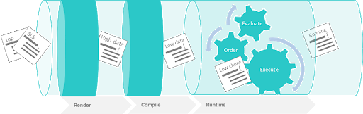
The runtime is a staged recursive algorithm that uses linear graph traversal to evaluate all requisites. This means:

1. Evaluate Chunk; the evaluation stage checks if requisites exist and reconciles them all.

2. Execution; the individual state executions happen.

The running dictionary

The state runtime is managed through a running dictionary. The running dictionary is used to track the execution of state runs. This structure is also the structure returned when the state run has finished. The running dictionary contains the returned information from the individual state function:

• a tag string

• __id__

• __run_num__

• name

• changes

• comment

• duration

• start_time

• result

The state of the running dictionary during the runtime is a cornerstone to the overall execution of states, and the evaluation of requisites.

The tag string

If the state system is executed without applying the highstate outputter a string is seen which displays a strange syntax. This syntax is a four field string delimited by a unique sequence, the _|-. This string contains the state, id, name, and function of the state that was executed:

STATE_|-ID_|-NAME_|-FUNCTION:
file_|-ldap_client_|-/etc/openldap/ldap.conf_|-managed:

The use of a string like this as the dictionary key for the running dictionary allows for the requisite system and the runtime to quickly and reliably look up required and already executed states.

The reason the tag string is not a tuple is that Salt is made to be JSON serializable and JSON does not support tuples as dictionary keys. The default outputter for the state runs is highstate not nested.

This outputter orders the output by the __run_num__ key in the running dictionary. The following state running dictionary is formatted by the highstate outputter as:

ID: ldap_client
Function: file.managed
Name: /etc/openldap/ldap.conf
Result: True
Comment: File /etc/openldap/ldap.conf updated
Started: 14:51:37.484849
Duration: 78.147 ms
Changes:
---------
  diff:
  ---
  -BASE dc=widget,dc=com
  -URI ldap://ldap.widget.com
  +BASE dc=acme,dc=com
  +URI ldap://ldap.acme.com

The tag string can be viewed by switching to another outputter such as the YAML outputter:

web:
  file_|-ldap_client_|-/etc/openldap/ldap.conf_|-managed:
    __id__: ldap_client
    __run_num__: 2
    changes:
      diff: "BASE dc=widget,dc=com\nURI ldap://ldap.widget.com\nBASE dc=acme,dc=com\nURI ldap://ldap.acme.com"
    comment: File /etc/openldap/ldap.conf updated
    duration: 78.147
    name: /etc/openldap/ldap.conf
    pchanges: {}
    result: true
    start_time: '14:51:37.484849'

Ordering states

The low state is an ordered list of low chunks. Now that it has been compiled the correct order needs to be applied. Requisites are not evaluated yet.

This ordering sequence orders the low chunks in this descending priority:

1. order flag: the order flag number, those applied by the state auto order systems and those applied manually by end users

2. Lexicographically via state: the state name, such as pkg, service, etc. are prioritized next.

3. Lexicographically via name: the name of the state declaration

4. Lexicographically via function: if names conflict then the function being called is the final lexicographical check

Start the runtime

Each execution in the runtime is called a “lowchunk” or a chunk of Salt low data. Now that the low state has been compiled, the time has come to begin the runtime execution. Since the low state is an ordered list of low chunks, or python dictionaries each representing a function call, the execution of the runtime begins with the evaluation of each low chunk in order.

Runtime evaluation

The state runtime evaluation is broken into two main routines, evaluation and execution. The evaluation routine checks for a number of conditions:

1. Verify that this chunk has not already been executed

2. Checks for requisites, if no requisites then execute

3. Checks that all requisites have executed, if requisites have not executed, evaluate them

4. Checks that all requisites have succeeded, if any failures are found do not evaluate. In the evaluation phase the requisite chain under the given low chunk is fully evaluated.

When a state is found with a requisite the required state is evaluated. If that state has a requisite then its requisites are evaluated until a state is found without requisites or all requisites have been executed.

Once the base of the chain is discovered then the chain is unraveled, executing each low chunk up until reaching the top of the requisite chain and finally executing the initial low chunk.

Runtime execution

1. When a low chunk is executed a number of checks are run:

   1. Add the __run_num__ value, this keeps track of the order in which the individual states were executed.

   2. The check_refresh method is called, this checks to see if the module loader system needs to be re-run before calling the state. Since installed packages and files may have made more state and execution modules available before this low chunk should be executed.

   3. Inject the __low__, __running__, and __lowstate__ values. These are the live data structures being used by the state runtime. They are made available to state modules to facilitate cross-module states.

2. The state function is then called, the code defined in the python state module is executed and the return value is tagged and added to the running dictionary.

Function call

The lowest layer of functionality in the state system is the direct state function call. State executions are executions of single state functions at the core.

These individual functions are defined in state modules and can be called directly via the state.single command:

salt '*' state.single pkg.installed name='vim'

Summarizing the state processing routines

The Salt state system provides a reliable process of evaluating state files so that they evaluate accurately and consistently: